Assignment 3 - Graphs in the xb Plane

Faith Hoyt

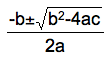
First, we want to consider the equation . Notice, that both our a and c values are fixed at one, but our b is going to be variable. In this case, we want to look at the xb plane. By using this, we can investigate the roots of a quadratic equation. Let's generalize this even further. Our most general form of the quadratic equation is . Recall that a root (also known as the zeros of a function) are the values where the equation is satisfied. By the fundamental theorem of algebra, we know that every polynomial of degree n has exactly n complex roots. We can find these roots by using the quadratic formula, where the radicand, , call tell us which of our roots are real and which ones are imaginary. Now, let's look and see how b changes our polynomial and our resulting roots. Let's first look at a graph where we just have b changing.

Notice, as b varies, the graph seems to give us a locus of what looks like another parabola. Depending on the sign of b, the graph goes through the bottom two quadrants. When b is positive, it goes through the third quadrant, or the negative side of the x axis and when b is negative it goes through the fourth quadrant, or the positive side of the x axis.

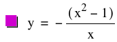
Now, we will look at the parabola in the actual x-b plane. This puts our b value as our dependent variable and our x value as our independent variable. You could also look at this as the xy plane, as we will technically be using y in place of b for graphing purposes. Let's solve our general equation for b.

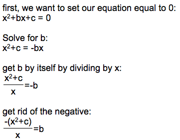
This gives us a rational equation we can use to graph for b and see better what it tells us about the roots. Let's first set c equal to 1.

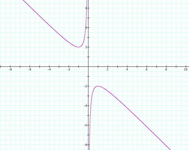
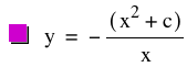
By looking at our graph above, we can see that when we set c=1, our range will be all real numbers except for . We can also observe that, much like our observation we made above with our general equation, when our x value is negative our y value (or b value) is positive. When our x value is positive, our y value (or b value) is negative.

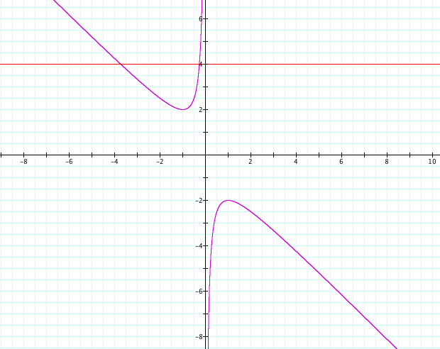
Now, let's take a given b. Let's first look at b=4.

When we look at our intersections of b=4 and our graph, we can see that our roots are approximately x = -0.268 and x = -3.732. We can find this by setting our two equations equal to each other. Now, we have graphed our equation that we were given in an x-b plane. So, rather than looking for our x-intercepts for our roots, as is given in the general definition of a root, we are looking for the intersections of our polynomial and our horizontal like of b =4, almost giving us a new coordinate system where b = 4 is like our x axis.

We can look at our system in motion to see how the "b-axis" varies.

So, for each value of b that we use (in this animation I have it set from -5 to 5), we will get a horizontal line. On a single graph, when we have b>2, we will get two negative real roots of the original equation. When b is equal to 2, we will get one real root, as the line will lie tangent to our graph. There will be no real roots for -2 < b < 2. When b = -2 there will once again only be one real root, as the line will be tangent to the graph again. And finally, when b < -2, we will have two positive real roots.

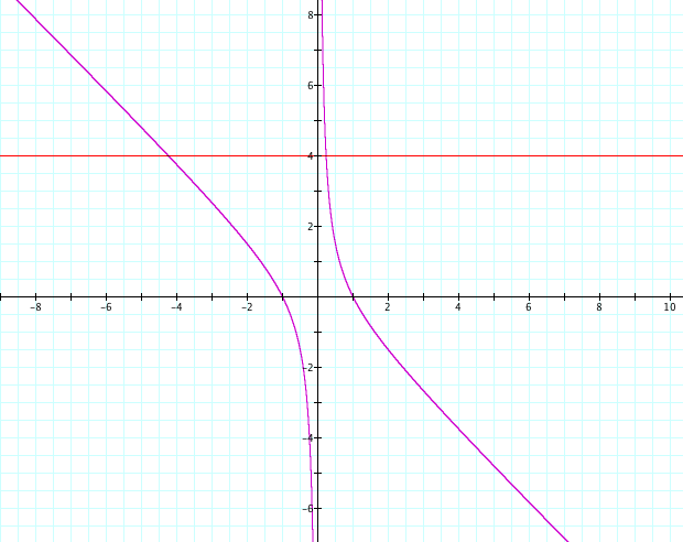
What happens if we were to change our c value? Let's investigate!! How about we try setting c = -1 rather than +1. Notice that we get a much different looking graph as a result.

Now, we can investigate the roots again. With this line, we can see that we have one positive real root and one negative real root at x = 0.236 and x = -4.236. Note that with this graph, we will always have two real roots.

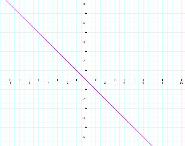
Let's look at one last value for c. What happens when c=0?

When we have c = 0, it appears that we have a linear equation as a result. However, note that in the fundamental theorem of algebra that every polynomial of degree n has exactly n complex roots. In this case, our degree is 2, thus meaning that we should have 2 roots. However, by looking at the graph, it appears that we only have one root. Thus, we must have one real root and one imaginary root.

We can combine these graphs to see how the roots correspond to each other:

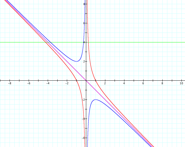
Now we can see the different number of roots that each graph has and how much c affects that number.

Go to my homepage